import numpy as np

class LinearSVM(object):
    def __init__(self):
        self.W = None
    
    def train(self, X, y, learning_rate=1e-3, reg=1e-5, num_iters=100,
              batch_size=100, verbose=False):
        """
        随机梯度下降法训练

        输入:
        - X:array(N, D)          训练数据, N 样本数, D 特征维度.
        - y:array(N, )           训练标签, y[i] = c 第 i 个样本的类别标签值
        - learning_rate:(float)  学习速率
        - reg:(float)            正则化参数
        - num_iters:(integer)    迭代次数
        - batch_size:(integer)   batch size

        输出:
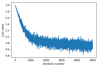
        - (list)                 每次迭代的损失值
        """
        # 探测 样本数, 维数
        num_train, dim = X.shape
        # 探测 标签数
        num_classes = np.max(y) + 1
        
        # 初始化参数
        if self.W is None:
            self.W = 0.001 * np.random.randn(dim, num_classes)
            
        # 迭代优化
        loss_history = []
        for it in xrange(num_iters):
            # 根据 batch size 随机取样 X_batch (dim, batch_size) y_batch (batch_size,)
            idx = np.random.choice(num_train, batch_size, replace=True)
            X_batch = X[idx]
            y_batch = y[idx]

            # 计算损失值和梯度
            loss, grad = self.svm_loss(X_batch, y_batch, reg)
            loss_history.append(loss)
            # 更新参数
            self.W -= grad *learning_rate
            
        return loss_history

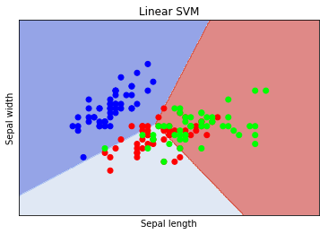
    def predict(self, X):
        """
        使用训练好的模型预测标签

        输入:
        - X:array(N, D)          训练数据

        输出:
        - y_pred:array(N, )      模型预测标签
        """
        y_pred = np.zeros(X.shape[1])
        scores = X.dot(self.W)
        y_pred = scores.argmax(axis=1)
        
        return y_pred
    
    def svm_loss(self, X, y, reg):
        """
        计算损失函数和梯度

        输入:
        - X:array(N, D)         训练数据
        - y:array(N, )          训练标签
        - reg:(float)           正则化参数

        输出:
        - (loss, gradient)      损失值, self.W的梯度. 
        """
        # 计算得分
        scores = X.dot(self.W)
        # 取出正确分类的得分
        correct_class_score = scores[np.arange(y.shape[0]), y].reshape(y.shape[0],1)
        
        # soft margin 计算 hinge loss
        margins = np.maximum(0, scores - correct_class_score + 1)
        loss = np.sum(margins) - y.shape[0]
        loss /= y.shape[0]
        
        # 正则损失
        loss += 0.5 * reg * np.sum(self.W * self.W)
        
        # hinge loss 梯度
        matrix = np.zeros((y.shape[0], self.W.shape[1]))
        matrix[margins > 0] = 1
        matrix[range(y.shape[0]), list(y)] = 1 - np.sum(matrix, axis=1)
        
        # 加上正则化梯度
        dW = (X.T).dot(matrix)/y.shape[0] + reg*self.W

        return loss, dW

# 导入数据
import matplotlib.pyplot as plt
from sklearn import datasets

iris = datasets.load_iris()
X = iris.data[:, :2]
X -= np.mean(X, axis=0)
y = iris.target

# 训练模型
svm = LinearSVM()
hist = svm.train(X, y, learning_rate=1e-3, reg=1e-7, num_iters=5000, batch_size=100, verbose=False)

plt.plot(hist)
plt.xlabel('Iteration number')
plt.ylabel('Loss value')
plt.show()

h = 0.01

x_min, x_max = X[:, 0].min() - 1, X[:, 0].max() + 1
y_min, y_max = X[:, 1].min() - 1, X[:, 1].max() + 1
xx, yy = np.meshgrid(np.arange(x_min, x_max, h),
                     np.arange(y_min, y_max, h))

Z = svm.predict(np.c_[xx.ravel(), yy.ravel()])

Z = Z.reshape(xx.shape)
plt.contourf(xx, yy, Z, cmap=plt.cm.coolwarm, alpha=0.6)

plt.scatter(X[:, 0], X[:, 1], c=y, cmap=plt.cm.brg)
plt.xlabel('Sepal length')
plt.ylabel('Sepal width')
plt.xlim(xx.min(), xx.max())
plt.ylim(yy.min(), yy.max())
plt.xticks(())
plt.yticks(())
plt.title('LinearSVC (linear kernel)')

plt.show()